Intelligence from compression

9/27/2025

Compression is Learning

Great theories often seem obvious once they click. I recently had that moment with the idea that compression is a form of learning. When this concept finally sank in, I began noticing it everywhere—especially in the foundations of today’s AI revolution. This felt so intuitive and exciting that I needed to regurgitate it, so it goes.

A JPEG Thought Experiment

If you’ve ever saved a photo on your phone, you’ve used JPEG. It’s an amazing program that lets you save your beautiful photos without eating up all your storage.

Take a raw 4K photo and ask, “How do I shrink it to a smaller image while still appearing the same to the naked eye?” Under the hood, the JPEG codec breaks a photo into small tiles, summarizes each tile into “broad strokes”, rounds off the details the human eye can’t perceive well and packs what’s left efficiently. Effectively, JPEG encodes knowledge about digital images, visual patterns, and human perception, allowing it to compress images intelligently. That knowledge is a form of intelligence—the rules the program must internalize so it can compact an otherwise massive bitstream.

To make this idea clearer and more generalizable, let’s use symbols to quantify the amount of information being learned. We’ll say that there’s a measure called $description\ length (L)$ that can be used to quantify how many “bits of information” something contains. A thing’s size is then $L(thing)$.

Now we can say that the JPEG program has a size of $P$, and the data that is all of the images in the world have a size of $M = L(raw\ images)$, and the resulting data from all of the compressed images have a size of $N = L(jpeg\ images)$.

I claim that the better the compression (smaller $N + P$), the more structure the program has captured, hence the more intelligent the program is. Why is this intuitively true?

• the simplest program just stores the raw $(N = M, P = 0)$, capturing no intelligence.
• A smarter program counts unique colors and stores them as a palette $N < M, P > 0$, encoding knowledge of digital images
• An even smarter one discards subtle colors and blurry details humans can’t perceive, encoding images very compactly ($N ≪ M, P\ moderate$), demonstrating a deeper understanding of human perception

So for the world’s image dataset $M$, the best compression (smallest $N + P$) within that setup corresponds to the program that captures the shared structure across $M$.

• intuitively this is because the program must learn the common patterns, correlations, and invariants that hold across the dataset to compress it well.
• an unintelligent, overfitting program that memorizes more data VS rules, and needs a larger P to store all those exceptions, which is inefficient.
• an unintelligent, underfitting program might be too simple, which cannot exploit the shared structure of the dataset, leading to a large $N$.

Knowing this, how do we find the "best compression" of some set of data?

Kolmogorov Complexity & MDL 101

With a dataset $D$, Kolmogorov complexity $K(D)$ is the $length$ of the shortest Turing program that outputs $D$ and halts. This is the best compression of the dataset, but we cannot compute this in practice. In practice, we find a model $M$ that encodes the dataset $D$. Once we've chosen a model, we can actually compute and optimize its description length.

Formally, this is the Minimum Description Length (MDL) principle. The MDL of a dataset $D$ is expressed as $L(D) = L(model) + L(data \mid model)$, where $L(data \mid model)$ captures the $length$ of the dataset under the model. This model often isn’t capable of recreating the dataset by itself, and therefore has some amount of error, so the term $L(data | model)$ actually also includes the error to bridge this gap.

From here on, just like in related literature, we’ll use description length and codelength interchangeably.

Also, a quick change: instead of representing datasets as $D$, let’s start thinking of them as distributions, where events in $D$ are drawn from a distribution $p$. This gives us a clean way to think about the information in a dataset, without being concerned about what the dataset consists of.

A quick detour to Entropy

How do we actually describe the codelength of a distribution $p$?

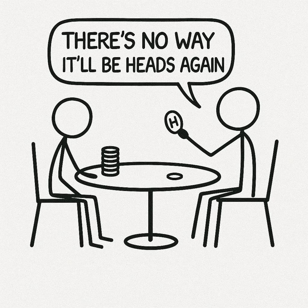
Let’s see this from an example where we have to encode a sequence of 100 coin flip events, given some probability distribution $p$

• For a fair coin ($p(heads) = p(tails) = 0.5$): we require 1 bit per flip because each outcome is maximally uncertain.
• Biased coin ($p(head) = 0.9$, $p(tail) = 0.1$): we only need ~0.47 bits per flip, since heads dominates and the code can compress long head runs aggressively.
• Extremes ($p = 0$ or $p = 1$): we don’t need any information (0 bits!) since every event is predictable.

Try to understand this intuitively! With a biased coin (90% heads), encoding a 100-flip sequence that is mostly heads requires much fewer bits because we just have to know which 10 positions are tails, since the rest are implicitly heads.

Formally, we call this the entropy of a distribution $p$, known as $H(p)$, and this is the average codelength required to transmit an event $x$ drawn from $p$ when using the best possible code.

$H(p) = -\sum_x p(x) \log_2 p(x)$

The more random the data, the higher the entropy!

Modern ML as Compression

Model training searches for a compact, parameterized program that compresses data well. Every training step tries to reduce how many bits you’d need to describe future examples, which makes predictions easier, more accurate, and more useful in practice.

As a reminder in MDL language:

$L(\text{dataset}) = L(\text{model}) + L(\text{dataset} \mid \text{model})$

• $L(\text{model})$ is how many bits I need to describe the architecture, priors, and specific weight instantiation.
• $L(\text{data} \mid \text{model})$ is the expected codelength to transmit the dataset using the model’s probability assignments.

If our dataset $D$ is drawn i.i.d. from a distribution $p$, then it has entropy $H(p)$. Our goal is to produce a model $q$ that emits the same distribution, so in expectation over the data, the information needed to recreate $p$ given $q$ is expressed below:

$H(p, q) = H(p) + KL(p \| q)$

where $KL$ = difference in distribution between the true distribution $p$ and model $q$, otherwise known as the Kullback-Leibler divergence.

So how do we optimize our model?

This is how we get to our loss term, which is almost exactly what we use to measure the performance of our LLMs today!

💡 Very loose derivation, meant to provide an intuition!

The entropy of the true distribution is $H(p)$. This is the irreducible baseline.

**The cross-entropy under a model distribution $q$ : $H(p, q) = \mathbb{E}{x\sim p}[-\log_2 q(x)]$.

Remember that the entropy of the true distribution $p$ under $q$ is $H(p, q) = H(p) + KL(p \| q)$, and because $H(p)$ is fixed, training can only reduce $KL(p \| q)$ by improving $q$. Thus, minimizing cross entropy loss is equivalent to minimizing the KL divergence $KL(p||q)$, since the true distribution’s entropy $H(p)$ is fixed

In practice, we also must consider our MDL principles to keep our model codelength smaller, so as described below, we must apply some tricks to keep our $L(model)$ small.

Shrinking the Model Term

You might wonder how a model with billions or trillions of parameters could possibly represent compression, since that’s a huge amount of data, but billion-parameter models don’t imply billions of information bits. $L(\text{model})$ depends on the built in assumptions (prior) and the precision needed to specify the final weights. The actual bits of information in huge models can be surprisingly small due to this prior (architectures), regularization, and clever optimization techniques. Here are some examples:

• In convolutional neural nets (CNN) for images, the architecture bakes in “locality via weight sharing”, where spatially close pixels are related in images, so the model doesn’t have to relearn that relationship
• The (self) attention mechanism in the transformer architecture ensures that “tokens look at other tokens to decide how much they matter right now” so the models don’t need to capture that relationship, for every possible dependency, in separate learned weights
• Regularization (e.g. L2 / weight decay to prefer smaller weights) sparsity, and quantization all reduce the effective bits needed to specify the learned parameters.
• Smart ways to initialize the parameters, and optimizer dynamics (e.g., SGD with momentum) steer parameter updates toward smoother, simpler solutions, which again lowers the descriptive cost.

In practice, working inside a well-designed architecture means $L(\text{model}) \ll (\#\text{weights} \times n \text{ bits per weight})$. The "code" the model transmits is closer to "which region of weight space, under these priors, explains the data".

Compression is the path to AGI

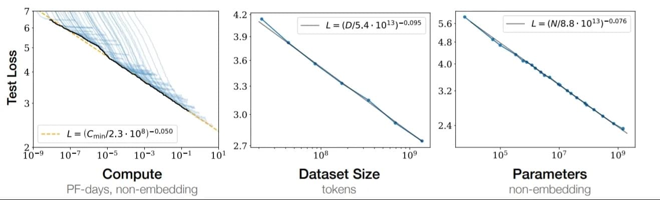
The most powerful illustration of this is scaling laws, which essentially represent compression curves.

On the dataset $D$ that encodes all of human knowledge and behavior in language, we see that as we scale models, data, and compute, the test cross-entropy consistently drops. This means the model gets better at representing the true distribution of human knowledge. In short: scaling up model parameters lets us find shorter and shorter descriptions of the same data, suggesting that we can scale our way to smarter compression, and thus toward genuinely intelligent models.

Of course, we don’t know where the limit is yet, as true Kolmogorov complexity for this dataset $K(D)$ is uncomputable, and we don’t yet know if stochastic gradient descent can ever reach that ideal form of compression. How close do scaling laws push us toward that theoretical limit $K$, and will that $K$ get us to AGI? We don’t know, but this is our clearest path there, and I am optimistic.